Observed Events Curve - Shifting About Redshift (Including an Alternate FUGE-like Universe)

I tried calculating redshift in a FUGE universe, and ran into what looked to be a problem.

My logic was as follows: if we are observing a photon from an event that occurred a time t ago, then that photon had a proper distance of x'=x.(ct₀-x)/ct₀ and the event location (at the time of observation) will be x=ct from the observation location.  So for any arbitrary wavelength of the photon:

1+z=λ_observed/λ_emitted=x/x'=ct₀/(ct₀-x)

z=ct₀/(ct₀-x)-1=(ct₀-(ct₀-x))/(ct₀-x)=x/(ct₀-x)

z=t/(t₀-t)

The problem is that using this equation, redshift for the CMB does not come out to be what is generally attributed to it (z_CMB=1100).  Recall that t₀ here is the age of the universe and t is the transit time for an observed photon (see most recent posts, particularly Mathematics for Taking Another Look at the Universe), so for a photon emitted during recombination, the event (also confusingly known as decoupling) that led to the CMB when the universe was 380,000 years old, t_CMB=(13.8×10⁹-380,000) years and:

z_CMB=t_CMB/(t₀-t_CMB)

z_CMB=(13.8×10⁹-380,000)/(13.8×10⁹-(13.8×10⁹-380,000))=36,300

This is 33 times higher than the standard answer.  We can reorganise the equation above to work out how old the universe must have been for photons from the CMB to have a redshift of z=1100.  Using æ_CMB=t₀-t_CMB (and thus t_CMB=t₀-æ_CMB):

z_CMB=(t₀-æ_CMB)/æ_CMB=t₀/æ_CMB-1

t₀/æ_CMB=z_CMB+1

æ_CMB=t₀/z_CMB+1

For z_CMB=1100, we get an æ_CMB=1.25×10⁶ years.  Hm, it appears that something is not right.

---

The question that immediately arises, at least for me, is how do we know that the redshift for photons from recombination is 1100 and how do we know that recombination happened when the universe was 380,000 years old?  And what are the error bars associated with these values?

The redshift value is a little rubbery, but is usually quoted as simply 1100, although it’s probably a bit lower.  Rhodri Evans (astrophysicist and author of The Cosmic Microwave Background - How It Changed Our Understanding of the Universe) has a blog post on the CMB redshift which gives a bit of the history, indicating that the value comes from a comparison between the temperature of the CMB radiation today and that at the time of recombination, so:

z_CMB=T_recomb/T_now=3000/2.725≈1100

This equation is a slight approximation, since it should be z+1=T_recomb/T_now and I will be using the non-approximation from now on.

Note also that the equation does not explicitly rely on the timing of the event.  The recombination is thought to have happened when the universe got sufficiently cool, so the timing isn’t actually key.  While Evans does write that “as the Universe expands, the temperature (..) decreases in inverse proportion to its size. Double the size of the Universe, and the temperature will halve”, to know when the temperature of the universe was 3000K, we would have to know what the temperature was at some other time, what that time was and what the relevant expansion rate was.

Note that in a FUGE universe, the radius of the universe is directly proportional to its age (so currently r₀=ct₀).  So, noting the inverse relationship, we could simply replace T_recomb and T_now with 1/æ_recomb=1/380,000 years and 1/æ_now=1/t₀=1/13.8×10⁹ years.  Which gives us … z≈36,300.

So, I still have questions about timing and redshift and now also temperature.

---

When I expanded my search to find out how the relevant temperatures are calculated, I stumbled on what looks to be a variant of the FUGE universe, described in papers that have been published in what appear to be legitimate journals.  This model is referred to more frequently as Flat Space Cosmology, but there are also references to “r_H=ct models” (presumably those similar to Melia's, where t is the age of the universe) and “growing black hole models” which seems to describe something akin to the FUGE universe (I disagree with the terminology but that may just be a matter of perspective).

Espen Haug and Eugene Tatum (and others) have, in the past half a year, published a number of papers, for the most part on open archive sites but sometimes in journals (for example the International Journal of Theoretical Physics).  The paper that most attracted my attention provides a method for calculating temperature, Solving the Hubble Tension by Extracting Current CMB Temperature from the Union2 Supernova Database (available from HAL open science, which is an open archive).

I’m not going to get into whether or not they have actually solved the Hubble Tension, instead I am going to look at equations in that paper that I have issues with.

The first appears late in the paper:

The complexity of this equation does not appear justified, since it resolves to:

Ʊ=2(4π/T_P)²/t_P

where T_P is Planck temperature and t_P is Planck time.  This follows from T_P=E_P/k_b where E_P=m_Pc² is Planck energy and k_b is the Boltzmann constant, noting that m_P=√(ħc/G), so that:

Ʊ=k_b²32π²G^1/2/c^5/2ħ^3/2=((E_P/T_P)².2.(4π)²/c²ħ).√(G/ħc)

Ʊ=((m_Pc²/T_P)².2.(4π)²/c²ħ)/m_P=(m_Pc²/ħ).2.(4π)²/T_P²

Ʊ=(√(ħc/G).c²/ħ).2.(4π/T_P)²=(√(c⁵/ħG).c²/ħ).2.(4π/T_P)²

And since t_P=(√(ħG/c⁵):

Ʊ=2.(4π/T_P)²/t_P=2.923×10^-19K^-2s^-1

This “composite constant” upsilon, which has no other apparent name than the Latinised Greek letter used to denote it, has no other apparent use than in the equation H₀=ƱT₀², where T₀ is the (current) temperature of the CMB.  In the paper in which upsilon is introduced, Upsilon Constants and Their Usefulness in Planck Scale Quantum Cosmology, it is derived purely from this simpler relationship.  (I should provide a warning here that SCIRP is considered to be a predatory publisher, meaning that there is no peer review for articles which are published after payment.  Tatum indicates that he consulted Dr. Rudolph Schild of Harvard-Smithsonian Center for Astrophysics.  Unfortunately, Schild apparently publishes in a fringe (and allegedly predatory) astronomy journal, Journal of Cosmology, of which he is the editor in chief.  Tatum has published in that journal at least twice.  That all said, if the mathematics is correct, it is correct irrespective of where it has been published, even if the author paid to have it published.)

Earlier in Solving the Hubble Tension by Extracting Current CMB Temperature from the Union2 Supernova Database, there was something that really attracted my attention, an equation for the current CMP temperature T₀:

Once again however, this can be simplified.  Note that R_H=c/H₀ is the Hubble radius which, in a flat universe, is equal to R_H=æ.l_P, and that l_P=√(ħG/c³) so:

T₀=ħc/(4π.k_b.√(æ.l_P.2.l_P))=ħc/(4π.(m_Pc²/T_P).l_P.√(æ.2))

T₀=ħc/(4π.(√(ħc/G).c²/T_P).√(ħG/c³).√(2æ))

T₀=T_P/(4π.√(2æ))

Meaning that the only equation in which upsilon is used, H₀=ƱT₀², resolves to:

H₀=ƱT₀²=2.(4π/T_P)²/t_P.(T_P/(4π.√(2æ))²

H₀=1/(æ.t_P)

This is precisely what one would expect from a flat universe.

There is a slightly different approach, just using R_H=H_o.c, but it is messy. 
This messiness can be alleviated if we work with T₀², so that:

T₀²=(ħc/(4π.k_b.√((c/H_o).2.l_P)))²=ħ²c²/((4π)².k_b².((c/H_o).2.l_P))

T₀²=ħ²c²/((4π)².(m_Pc²/T_P)².((c/H_o).2.√(ħG/c³)))

T₀²=ħ²c²/((4π)².(m_P²c⁴/T_P²).((c/H_o).2.√(ħG/c³)))

T₀²=ħ²c²/((4π)².((ħc/G).c⁴/T_P²).((c/H_o).2.√(ħG/c³)))

Then rationalising and rearranging

T₀²=√(ħG/c⁵).H_o/(2.(4π)²/T_P²)=t_P.H_o/(2.(4π)²/T_P²)=H_o/Ʊ

So, of course, H₀=ƱT₀².

---

A potential critique, if one were to only consider Solving the Hubble Tension by Extracting Current CMB Temperature from the Union2 Supernova Database, is that all Haug and Tatum have done here is shuffle numbers around in order to hide H₀ in T₀, and then created a new constant (Ʊ) which does nothing more than reveal the previously hidden H₀.  While that may appear to be the case, such critique ignores the fact that T₀ is a measured value, specifically the temperature of the CMB today or 2.72548±0.00057 K (from 2009 but seemingly still most commonly used).  As Tatum showed in Upsilon Constants and Their Usefulness in Planck Scale Quantum Cosmology, upsilon can be used to extract H₀ from the CMB temperature:

ƱT₀²=(2.923×10^-19K^-2s^-1).(2.72548K)²=2.171×10^-18s^-1

Noting the km to Mpc ratio, 3.086×10¹⁹km/Mpc, we find:

ƱT₀²=66.99km/s/Mpc≈H₀

This would correspond to a FUGE universe which is 14.60 billion years old.

---

The equation for T₀ was presented in a slightly different format in an earlier paper by Tatum, Seshavatharam and Lakshminarayana The Basics of Flat Space Cosmology:

Why the third term is there is beyond mjue, given the parallels between the second and the fourth.  The first two terms are a modification to the Hawking radiation temperature equation, as Tatum acknowledges in Upsilon Constants and Their Usefulness in Planck Scale Quantum Cosmology, (noting that k_b is the same thing as k_B).  The standard Hawking radiation temperature equation:

The implication here is that Tatum et al. are conceptually equating the temperature of the CMB to the temperature of a black hole with the same radius, but with a different value for mass – which doesn’t make sense because with a different mass you are no longer talking about a black hole.  Alternatively, they are effectively scaling that temperature (and the expression of mass in their equation as being less than that of an equivalent Schwarzschild black hole is misguided).

This leads to an intriguing notion and the potential for a different approach, in terms of establishing redshift.

Consider the Hawking radiation temperature for a black hole with the mass and radius of the prevailing Hubble sphere, now and at the time of recombination (when the CMB was generated).  Recall that, per Carroll, “a spatially flat universe remains spatially flat forever” and “the corresponding Schwarzschild radius … equals the Hubble length”.  As a consequence, the radius of the universe now is r_H-0=c/H₀ and, at recombination, it would have been r_H-recomb=c/H_recomb, where H_recomb is Hubble parameter for that time. 

According to Andrei Starinets’ General Relativity and Cosmology solution notes, the Hubble parameter at recombination (note that the event is referred to in the notes as “decoupling”) is H(t_d)=H_recomb= H₀.1000√1000.  Noting that Schwarzschild radius is directionally proportional to mass, and Hawking radiation temperature is inversely proportional to radius, we have (per the equation above from Rhodri Evans, without the approximation):

z_CMB+1=T_H-recomb/T_H-0=r_H-0/r_H-recomb=(c/H_now)/(c/ H_recomb)=H_recomb/H₀

z_CMB+1=1000√1000=31,600

Hm, still not right but it is closer to my answer but given that a(t₀)/a(t_d)=1000 should be almost certainly thought of as a(t₀)/a(t_d)=10³, rather than a(t₀)/a(t_d)=1.000×10³.   The tutorial notes go on to state that:

So, if we plug in the values t_d=380,000 years and t₀=13.8×10⁹ years, we get:

Curiously, if a(t₀)/a(t_d)=1100 is used, we get z=36,000.  It is interesting to note that the common rendering of is z_CMB=1100, but from the above this appears just be the ratio of scale factors, or there's an issue with Rhodri Evans' equations.  If not, is there some widespread blurring between the ratio of scale factors and redshift z or is Starinets making a mistake in his solution notes?

Note also that the solution notes do something akin to a pea and cup trick (similar to Tatum’s apparent hiding and revealing of H₀ above).  He presents three equations:

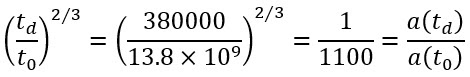
a(t_d)=a(t₀)/1000 … H(t_d)= H₀1000√1000 … (t_d/t₀)^2/3= a(t₀)/a(t_d)=1/1000

It is not difficult to see, when these equations are put side by side to see that:

H(t_d)/H₀=1000^3/2 and t₀/t_d=1000^3/2

So:

H(t_d)/H₀=t₀/t_d

It is unclear why this much simpler and, in retrospect, obvious relationship is not used.

We can go further to show that, since H(t_d)=H_recomb, t_d=t₀-t_CMB (where t_CMB as defined above is how long ago the CMB was generated) and z_CMB+1=H_recomb/H₀:

 z_CMB+1=t₀/(t₀-t_CMB)=t₀/(t₀-t_CMB)-(t₀-t_CMB)/(t₀-t_CMB)+1=t_CMB)/(t₀-t_CMB)+1

And generalising:

z=t/(t₀-t)

Which is the result that I arrived at, using a second approach

---

Another approach is on the basis of a FUGE universe using Evan’s equation z_CMB=T_H-recomb/T_H-0.

In a FUGE universe, the current mass is M(t₀)=(m_P/2)t₀/t_P and at any time t ago, M(t)=(m_P/2).(t₀-t)/t_P.  Noting that mass is directly proportional to Schwarzschild radius and temperature is inversely proportional to radius, the equation above becomes:

z+1=T_recomb/T_now=M(t₀)/M(t_CMB)=((m_P/2)t₀/t_P)/((m_P/2).(t₀-t)/t_P)

z+1=t₀/(t₀-t)=t₀/(t₀-t)-(t₀-t)/(t₀-t)+1=t/(t₀-t)+1

This is precisely what I arrived from Starinets solution notes, so we have the same result using a third (slightly different) approach.

---

In Solving the Hubble Tension by Extracting Current CMB Temperature from the Union2 Supernova Database, Haug and Tatum get a third value for z.  This is established from use of his (apparently) scaled temperatures.  This ends up with him comparing T₀=T_P/(4π.√(2æ₀)) with T_CMB=T_P/(4π.√(2æ_CMB)) so, noting that the subscript CMB here is equivalent to recomb used above:

z+1=T_CMB/T_now=T_recomb/T_now=(T_P/(4π.√(2æ₀)))/(T_P/(4π.√(2æ_recomb)))

z+1=√(æ₀/æ_recomb)=√(t₀/(t₀-t))=√(36,000)

It should be noted that they state that there was a choice between T_t=T₀√(1+z) and T_t=T₀(1+z).  They chose the latter, but if we choose the former, we get:

z+1=(T_recomb)²/(T_now)²=(T_P/(4π.√(2æ₀)))²/(T_P/(4π.√(2æ_recomb)))²

z+1=æ₀/æ_recomb=t₀/(t₀-t)=t₀/(t₀-t)-(t₀-t)/(t₀-t)+1

z=t/(t₀-t)

So we have a fourth approach to arrive at the same result.

---

Finally, returning to Starinets’ solution notes, he notes that in the “matter-dominated era” a(t)=(t/t₀)^2/3.  This is a Standard Model thing.  In a FUGE universe, a(t)=(t/t₀) at all times, which is to say that there has been more stretching of the universe over the period between recombination and today and more redshift, so it’s precisely what we should expect.

---

As I have managed to find five* methods for arriving at equations for redshift which indicate that, for an event that occurred a period t ago, z=t/(t₀-t), I am no longer convinced that there is a problem with my calculations.

There is however some confusion on the part of Tatum et al. associated with the introduction of their “composite constant” upsilon.  This will be touched on again in the next (shorter) post.

---

* I understand that not all five methods are entirely distinct.  Also questions remain about Tatum's equations, not only with respect to his methods for getting the papers that contain them published but also with respect to whether the implied relationship he identifies via those equations is anything more than a rather startling coincidence.

Observed Events Curve - Hang On! Aren't I Double Dipping? (SPOILER - No, I am not.)

It could be argued that, in Observed Events Curve - Addressing a Point of Potential Confusion, I double dipped.

Note the argument involving a hypothetical racetrack along which a photon was approaching us (as observers).  I said that the location from which a photon would be travelling would recess away at a rate determined by its proper distance.  I effectively said that the photon would advance towards us at a rate given by c-v, where v is the speed of recession.  So, over an increment of time Δt, the photon would advance by (c-v).Δt.  During that increment of time, however, the entire racetrack will have expanded by a factor of (1+H(æ).Δt), where æ is the age of the universe (at that time, t).  Note that v=x'(t).H(æ), where x'(t) is the proper distance at t (and that the value of H(æ) will vary over the period Δt).

It could be argued that I used the expansion twice, first to retard the advancement of the photon and then to stretch the racetrack, pushing a sufficiently distant photon even further away than it started.

Well, yes, I did.  The question is whether this is valid.

I think it is. 

What this apparent double dipping is doing is accounting for the fact that the entirely of the metaphorical racetrack is expanding, but we have metaphorically put a pin in the observer’s location.  For a sufficiently long period ago, the proper distance to the location of the photon is small but the rate of expansion is great.

Speaking in terms of comoving distance, the photon is always advancing towards the observer.  For example, consider the cleaned-up chart in Observed Events Curve - Addressing a Point of Potential Confusion:

The purple dotted line illustrates the comoving distance to the location of the observed photon that it had at t=10,000 million years.  Note that the comoving distance is greater than any proper distance after the event and less than any proper distance before the event.  In that sense, the photon is always advancing on the observer, which is precisely what we would expect.  If we normalise the chart to consider distances from a comoving distance perspective, rather than the proper distance perspective above, we get this:

As could be expected, the photon actually advances towards the observer at a constant rate.  Which indicates that I was not, in fact, double dipping.

This graph also offer a different perspective on the underlying mathematics.  The events on the blue line are given by t.(c-v). Note the similarity of this equation in form to x'=ct.(ct₀-ct)/ct₀=x.(ct₀-x)/ct₀.

The implication, when understanding the nature of a FUGE universe, is that (in comoving terms) v=H₀.ct=ct/t₀, so:

t.(c-v)=t.(c-ct/t₀)=t.(ct₀-ct)/t₀=ct.(ct₀-ct)/ct₀=x.(ct₀-x)/ct₀=x'

Another Look at Taking Another Look at the Universe

In Mathematics for Taking Another Look at the Universe, I presented this chart (discussed further in Apparent Hubble Parameter Value), which plots the value of the Hubble parameter:

I should be explicit about how this chart was generated.  First, I should explain the calculations used in generating the chart discussed in Mathematics for Taking Another Look at the Universe, first introduced in Taking Another Look at the Universe:

This chart illustrates the proper distances (x') of a photon over time from the location of an observer at (x,t)=(0,0), in a FUGE universe of age t₀=13,000 million years, given that the photon is observed by that observer.

To generate the chart, I had three columns in a spreadsheet (the red line is actually just a line overlaid over the chart).  There was one for the x-axis, from 0 to 13,800 (millions of years) at intervals of 50, one for the blue curve (x'=(13800-x).x/13800)) and another for the grey line, from 13,800 (millions of light years) to 0 also at intervals of 50.

The blue curve plots every event through which a photon emitted very early in the FUGE universe’s chronology must pass in order to be observed.  That path is one through spacetime and has a spacetime length of 15,840 million (light) years.  This should be compared with a hypothetical static universe in which a photon reaching us after time t would have travelled across a distance of ct, so the magnitude of the spacetime distance would have been √2 times that.  Such a path could be normalised by merely multiplying by (distance/spacetime distance).

To generate the Hubble parameter chart, I replicated the first two of the three columns discussed above with the x value multiplied by 1.000001. Then I created a column each for Δt (s), Δx (km), x (Mpc), x_ST (Mpc) and Δx_ST (km).

The first column, Δt, contained only the equivalent of 0.000001 million years (4.3548×10¹¹ seconds) in every row.  The second, Δx, had the difference in the values of x before and after multiplication by 1.000001, expressed in km.  The third column merely converted the original values of x into Mpc.

The fourth and fifth columns, x_ST and Δx_ST, need some explanation.  They relate to the spacetime pathlength of a photon through all observable events, as represented above, that has a length of 15,800 million (light) years.  So, x_ST(t) is the length between x'(0) and x'(t), while Δx_ST is the delta between the x_ST(t₁) and x_ST(t₂) where Δt=|t₂-t₁|, where both are normalised in a similar way to as discussed above, specifically after division by 15,840 and multiplication by 13,800.

The Hubble parameter chart has two plots, a blue one and an orange one. The flat blue line results from the equations H₀=Δx/Δt/x=Δx_ST/Δt/x_ST=70.855 km/s/Mpc.  The orange curve plots apparent a hypothetical “apparent Hubble parameter” (H_App) from the equation H_App=Δx_ST/Δt/x, on which H_App varies between 70.855 and 87.143 km/s/Mpc.  (Note that if Δx_ST is not normalised, the H_App value ranges from 78.784 to 100.022 km/s/Mpc.  This is interesting, given that an H₀ magnitude of 100 appeared frequently before 2013, but that value should not be taken as meaningful, since 100 could be more realistically thought of as an order of magnitude, 10², rather than 1.00×10².)

In Apparent Hubble Parameter Value, I wrote “I cannot say with any confidence that the apparent acceleration of the universe (using recent measurements of nearer galaxies) is due to an artefact of measurement related to blending values of x=ct and x'.”  This still stands but note that, per the above, the use of x' not entirely accurate.  It’s really a blending of x=ct and x_ST.

Note that while I can’t say with confidence that a blending of x=ct and x_ST leads to apparent recent acceleration of the universe, because the evidence doesn't appear to exist, I can at least point to a mechanism by which measurement leads to it, as an artefact, rather than being a real thing.

Note also that what we have effectively been discussing above is the effect of recession on the location of an event.  What has not been discussed is how we, as observers, can determine speed of recession.  I’ll address that in the next post.

Apparent Hubble Parameter Value

In Mathematics for Taking Another Look at the Universe, I presented this chart:

Then, right at the end, I wrote: “I do acknowledge that the ‘Apparent’ values of H in the recent past/near vicinity are very high.  This is worthy of further investigation.”

The notion here is that, for closer events (in time and also space), the equation H=Δx'/Δt/x gives higher values of H.  For clarity, Δx' is the difference in proper distance over the period Δt for a location at an effective distance from an observer given by x=ct (where t is how long ago a photon would have had to have been emitted to be observed at the equivalent of t=0 [ie now]).

Note that this equation blends two variants of distance, so its use would be problematic.  Using the equation H=Δx/Δt/x results in the invariant H=70.855km/s/Mpc for all values of x=ct (the flat blue line).

I downloaded the NASA/IPAC Extragalactic Database list of galaxies to get an idea of what values of H were recorded to galaxies at various distances (and also redshift values).

Unfortunately, it appears that the value of H recorded appears to depend more on the paper from which it is extracted rather than the distance of the relevant galaxy.  H values range from as low as 42 to as high as 103, per the table below.

H	Year	Method	Ref Code	Galaxies (N)
103	1984 1985 1986	Tully-Fisher	1984A&AS...56..381B 1985A&AS...59...43B 1986A&A...156..157B	2073 887 398
100	1981 1992 2013	Tully-Fisher	1981ApJ...248..408D 1992ApJ...395..347B 2013ApJ...771...88L	303 35 568
100	1992	D-Sigma	1992ApJ...384...43G	35
100	1998	Magnitude	1998A&A...337...31R	72
100	2009 2010	GRB	2009EPJC...63..139W 2010JCAP...08..020W	32 19
95	1980	Tully-Fisher	1980ApJ...239...12A	40
95	1984	Faber-Jackson Tertiary	1984ApJS...56...91D	1104 278
92	1993	Tully-Fisher	1993AJ....105...97S	16
91	1984	Tully-Fisher	1984ApJ...278..475B	20
90	1985	Tully-Fisher	1985A&A...153..125G	257
88	1989	Faber-Jackson FP	1989ApJ...344L..57P	20 20
85	1995	Tully-Fisher	1995A&A...294L...9W	1
85	1992	Tully-Fisher	1992ApJS...81..413M	2711
85	1988	Tully-Fisher	1988ApJ...330..579P	40
85	1984	Sosies	1984ApJ...282..382P	17
84	1986	Tully-Fisher	1986AJ.....91.1286S	22
82	1997 1987	Tully-Fisher SNIa	1997ApJS..108..417Y 1987PASP...99..592P	207 1
80	1983	Tully-Fisher	1983ApJ...265....1A	44
77	2000 1994	Tully-Fisher	1994AJ....107.1962B 2000ApJ...533..744T	2 21
75	2016 2014 2013 2012 2012 2008 2006 2005 2002 2001 1994 1990 1986	Tully-Fisher	2016AJ....152...50T 2014MNRAS.444..527S 2013ApJ...765...94S 2012ApJ...749...78T 2012ApJ...749..174C 2008Ap.....51..336K 2006Ap.....49..450K 2005Ap&SS.298..577R 2002ApJ...565..681R 2001PhDT.......242M 1994A&A...283...21S 1990ApJ...351L...5W 1986A&A...164...17G	2306 3470 22 18 98 406 2724 2 1 23 64 2 2
75	1997	Tully-Fisher IRAS D-Sigma	1997ApJS..109..333W	8839 2946 1086
75	1988	Tully-Fisher Tully est	1988NBGC.C....0000T	942 1434
75	1997	FP	1997MNRAS.291..488H	22
75	1995	GRB	1995ApJ...453..583W	8
75	1991 1982	SNIa	1991AJ....102..208H 1982ApJ...254....1A	1 2
75	1982	CMD	1982AJ.....87..462G	2
75	1982	SZ effect	1982ApJ...257..473B	2
75	2010	GC radius	2010ApJ...715.1419M	1
74.4	2014	Tully-Fisher	2014ApJ...792..129N	110
74.4	2013	Tully-Fisher FP SBF Statistical TRGB SNIa Cepheids	2013AJ....146...86T	5851 1366 274 249 243 216 3
74.3	2015	L(Hβ)-δ	2015MNRAS.451.3001T	25
74.3	1983	Tully-Fisher	1983ApJ...275..430V	54
74.2	2011 2010	SNIa	2011A&A...526A..81B 2010ApJ...716..712A	26 687
74	2017	GRB	2017A&A...598A.112D	158
74	2012 2003	SNIa	2012ApJ...744...38F 2003AJ....125..166K	1 2
74	1996	Tully-Fisher	1996ApJ...463...60B	3
73.8	2017 2014	SNIa	2017JCAP...03..056C 2014ApJ...795...44R	19 335
73	2016 2011	SNII optical	2016AcA....66..219H 2011MNRAS.417.1417F	1 2
73	2015	Maser	2015ApJ...800...26K	1
73	2013 2012	SNIa	2013ApJ...777...40M 2012A&A...546A..12V	1 3
73	2011	Tully-Fisher	2011A&A...532A.104N	688
73	2010	GRB	2010JCAP...08..020W 2006astro.ph..9262M	12 24
73	2009	Cepheids	2009RoAJ...19...35A	93
72	2017	G Lens	2017ApJ...835L..25M	1
72	2015	FP	2015MNRAS.451.2723S	8
72	2015 2014 2013 2012 2011 2011 2010 2010 2010 2009 2009 2009 2009 2008 2008 2008 2007 2007 2006 2006 2006 2004	SNIa	2015ApJ...798...39M 2014ApJ...784..105W 2013ApJ...773...53F 2012ApJ...754...19M 2011ApJ...731..120M 2011AJ....141...19B 2010ApJ...721.1608B 2010AJ....140.2036S 2010AJ....139..120F 2009ApJ...704.1036F 2009ApJ...704..629M 2009ApJ...697..380W 2009A&A...505..265L 2008MNRAS.384..107E 2008ApJ...689..377W 2008AJ....136.1482S 2007AJ....133...58K 2007A&A...469..645S 2006ApJ...647..501P 2006ApJ...645..488W 2006AJ....131.1639K 2004ApJ...602..571B	1 108 79 20 110 33 17 15 28 56 39 3 1 1 44 3 1 1 90 98 3 58
72	2014	Tully-Fisher	2014Ap.....57..457K	145
72	2011	GeV TeV ratio	2011arXiv1111.0913P 2010MNRAS.405L..76P	18 17
72	2011 2010 2008	GRB	2011ApJ...736....7C 2010JCAP...08..020W 2008JCAP...07..004M	1 8 69
72	2002	D-Sigma	2002AJ....123.2159B	46
71.6	2014 2013	SNIa	2014ApJ...786....9P 2013ApJ...768..166J	10 1
71	2014	BL Lac Luminosity	2014A&A...565A..12P	3
71	2013 2011 2011	GRB	2013MNRAS.431.3550G 2011MNRAS.413.2173G 2011A&A...526A.153K	1 2 5
71	2010	SGRB	2010ApJ...709..664R	12
71	2005	HII LF	2005MNRAS.356.1117S	15
71	2001 1982	Tully-Fisher	2001ApJ...553...47F 1982PASAu...4..419V	36 11
70.8	2015 2008	SNIa	2015ApJS..219...13W 2008MNRAS.389.1577T	31 107
70	2018	SNIa SNIa SDSS	2018PASP..130f4002S	2795 3027
70	2018 2017 2016 2016 2015 2014 2014 2014 2013 2013	SNIa	2018ApJ...859..101S 2017MNRAS.464.4476C 2016JBAA..126..364F 2016ApJ...821..115W 2015ApJ...811...70R 2014MNRAS.438.1391P 2014AJ....148....1Z 2014A&A...568A..22B 2013MNRAS.434.1443X 2013MNRAS.433.2240G 2013ApJ...763...88C 2013ApJ...763...35R 2012MNRAS.426.2359M 2012ApJ...748..127F 2012ApJ...746...85S 2011ApJS..192....1C 2011ApJ...740...92G 2011ApJ...738..162S 2008ApJ...686..749K 2006A&A...447...31A 2000ApJ...539..658K 1992ApJ...400..127R 1987ApJ...315L.129F	847 4 1 345 4 60 1 740 48 583 1504 1 28 75 15 472 206 860 398 117 5 1 1
70	2017 2017	SNII optical	2017MNRAS.472.4233D 2017ApJ...835..166D	61 133
70	2017 2015 2015 2015 2014 2014 2013 2013 2013 2013 2012 2011 2009 2006	BL Lac Luminosity	2017ApJ...834...41K 2015arXiv150203012A 2015ApJ...799....7A 2015AJ....150..181L 2014ApJ...784..151S 2014A&A...570A.126L 2013ApJ...768L..31F 2013ApJ...766...35F 2013ApJ...764..135S 2013ApJ...764...57D 2012A&A...547A...1N 2011A&A...529A..49H 2009MNRAS.397L..55B 2006AJ....132....1S	5 2 1 1 11 2 1 1 1 1 1 1 1 4
70	2016 2015 2015 2015 2015 2014 2014	GeV TeV ratio	2016MNRAS.459.3271A 2015MNRAS.449.1018Y 2015MNRAS.447.2810Y 2015MNRAS.446..217A 2015ApJ...802...65A 2014PASJ...66...12Z 2014A&A...567A.135A	1 1 1 1 1 2 1
70	2016 2013 2013 2013 2010 2007 2004	GRB	2016MNRAS.458.3821U 2013A&A...551A.133P 2013ApJ...763..125M 2013A&A...552L...5P 2010JCAP...08..020W 2007ApJ...660...16S 2004AIPC..727...37A	19 1 1 2 2 69 42
70	2016 2014 2001	FP	2016A&A...596A..14S 2014MNRAS.445.2677S 2001MNRAS.321..277C	119078 8884 396
70	2015 2013 2012	SGBR	2015ApJ...808..190R 2013ApJ...766...41S 2012A&A...545A..77R	1 1 20
70	2014	G Lens Magnitude	2014ApJ...797...98L	20 22
70	2014	GeV TeV ratio BL Lac Luminosity	2014A&A...572A.121A	1 1
70	2012	G Lens	2012MNRAS.426..868S	1
70	2011 1999 1992	Tully-Fisher	2011A&A...531A..87I 1999AJ....118.1489D 1992ApJ...396..453H	42 111 33
70	1997	SZ effect	1997ApJ...481...35H	5
70	1988	D-Sigma	1988MNRAS.235.1177L	18
69.7	2010 2009	GRB	2010JCAP...08..020W 2009MNRAS.400..775C	18 152
69	1997	Tully-Fisher	1997MNRAS.290L..77S	3
69	1991	D-Sigma	1991BAAS...23..956G	5
68	1996	SNIa	1996ApJ...465L..83R	7
67	1996	SNIa	1996ApJ...457..500H	26
66	1994	SNIa	1994A&A...281...51M	13
65.2	1997	Tully-Fisher	1997A&A...326..915T	21
65	2010 2010 2009 2009 2007 2007 2007 2006 2006 2005 2004 2003 2003 2002 2001 2001 2001 2000 1998 1998 1998 1998 1996 1996 1996 1995	SNIa	2010arXiv1006.2112L 2010ApJ...708.1748F 2009ApJS..185...32K 2009ApJ...700.1097H 2007ApJ...666..694W 2007ApJ...659..122J 2007ApJ...659...98R 2006MNRAS.366..682S 2006ApJ...642....1C 2005AJ....130.2453K 2004ApJ...607..665R 2003ApJ...594....1T 2003ApJ...589..693B 2002ApJ...577L...1B 2001ApJ...560...49R 2001AJ....122.1616K 2001AJ....121.3127V 2000A&A...361...63T 1998ApJ...507...46S 1998ApJ...504..935R 1998ApJ...493L..53G 1998AJ....116.1009R 1996ApJ...473..588R 1996ApJ...473...88R 1996AJ....112.2398H 1995ApJ...445L..91R	249 2 576 1486 414 131 41 1 9 21 186 35 6 1 1 8 1 1 2 10 8 80 20 23 8 13
65	1999	GRB	1999ApJ...511L..79S	52
65	1980	Tully-Fisher Statistical	1980ApJ...238..458M	23 1
62.3	2008	SNIa	2008A&ARv..15..289T	20
60	2000	SNIa BCG	2000ApJ...540..634P	239 288
58	1997	Grav Stab Gas Disk	1997ApJ...485..439B	2
56	1992	SBF SNIa	1992ARA&A..30..359B	1 5
55	1984	Faber-Jackson	1984ApJS...56...91D	383
54	1997	Tully-Fisher	1997A&A...326..915T	21
53.9	1984	Tully-Fisher	1984A&A...132..253R	19
50	1996	FP SNII optical	1996MNRAS.280..167J	52 26
50	1994	SNII optical	1994ApJ...433...19S	2
50	1989	D-Sigma	1989ApJS...69..763F	798
50	1983	Tully-Fisher	1983A&A...125..187R	1
44	2007	AGN time lag	2007MNRAS.380..669C	14
42	1999	AGN time lag	1999MNRAS.302L..24C	1

Of all the papers listed (the Ref Code refers to papers), there are two that have more than one value of H for the galaxies surveyed.

1984ApJS...56...91D refers to A comparison of distance scales for early-type galaxies by de Vaucouleurs and Olson.  Looking through the paper, it does not appear that the Hubble parameter value was calculated.  Looking through the table above, two values are presented, H=95 and H=55 (km/s/Mpc).  Looking at the spreadsheet (NASA/IPAC Extragalactic Database (NED) list of galaxies) it can be seen that 284 entries have H=55 marked against them and 1382 entries have H=95.  However, there are not 1666 unique galaxies, only 425.  For every instance of H=55, there is at least one entry with H=95 recorded.  It’s extremely strange.

For example, for NGC 3619, there are two entries, one with H=55 and one with H=95.  However, the entry with H=55 has a distance of 44.7 Mpc and the entry with H=95 has a distance of 23.3 Mpc.  Similarly with NGC 3203 (D=20.3 and 37.8), NGC 3193 (various values of D from 14.7 through to 25.6 for H=95 and D=38.5 for H=55) and so on.

Given the age of the survey, 40 years ago now, and these peculiarities I’d suggest that we ignore it.

2010JCAP...08..020W refers to Observational constraints on cosmological models with the updated long gamma-ray bursts by Wei.  Again, the paper doesn’t specifically calculate the value of the Hubble parameter.  The NED list has 109 entries against this paper, covering 97 distinct galaxies of which only 46 have Hubble parameter values entered against them.  There does not seem to be any relationship between Hubble parameter and distance (despite Wei writing about “the discovery of current accelerated expansion of our universe”).  

The H values attributed to this paper vary between 100 and 69.7 km/s/Mpc.  At the upper range there are GRB 071020 (D=12,700 Mpc) and GRB 050904 (D=15,300 Mpc), with H=100 and H=69.7 respectively and towards the lower range there are GRB 010921 (D=1,620 Mpc) and XRF 040912 (D=1,760 Mpc), with H=73 and H=100 respectively.

So, while this paper is newer, at 14 years ago, it doesn’t seem to be aiming at establishing Hubble parameter values (but rather establishing the validity of the Gamma Ray Burst method, and filling in a gap in the data, referred to as a ‘desert’), and probably could be safely ignored.

That leaves all the other papers for which there is one value for the Hubble parameter, and one value only.

Interestingly, if we consider only the papers over certain period, the values for the Hubble constant calculated in the “wisdom of the crowd sort of way” (average of all values) are: past 40 years (1985-2024) – H=71.3, past 30 years (1995-2024) – H=70.87, past 20 years (2005-2024) – H=70.57 and past 10 years (2015-2024) – H=70.1.  I wouldn’t get too excited about the value zeroing in 70 since the spreadsheet generally seems to have a low level of specificity.  I think that 100 just means the value is considered to be somewhere between 50 and 150 (or even higher).  Similarly, 70 probably means something between 65 and 75.  There are more accurate values provided, for example 70.8, recorded against 2015ApJS..219...13W – First Results from the La Silla-QUEST Supernova Survey – and 2008MNRAS.389.1577T – Light-curve studies of nearby Type Ia supernovae with a Multiband Stretch method, but note that the authors in both instances set the value of H₀, they don’t calculate it.  This raises the question of whether, in the documents referred to the NED list, is H always an assumed value?  If so, then the list is of no use for what I am trying to establish.

As a consequence, there does not appear to be any supporting evidence, so I cannot say with any huge confidence that the apparent acceleration of the universe (using recent measurements of nearer galaxies) is due to an artefact of measurement related to blending values of x=ct and x'.  All there is is a potential mechanism.